

Export citation and abstract BibTeX RIS

Original content from this work may be used under the terms of the Creative Commons Attribution 4.0 license. Any further distribution of this work must maintain attribution to the author(s) and the title of the work, journal citation and DOI.
1. The warming Earth
The Earth is warming from human activities, primarily because of increases in carbon dioxide and other greenhouse gases (GHGs) in the atmosphere that reduce the outgoing infrared radiation from the planet escaping to space. This creates an energy imbalance at the top-of-atmosphere (TOA) called Earth's energy imbalance (EEI). It creates heating of the planet, which is manifested in multiple ways, only one of which is the rise in global mean surface temperature (GMST) (figure 1). The latter has been the primary focus for tracking global warming and 2021 was rated as the fifth or sixth highest on record, but the top 8 warmest years have all occurred since 2013 (figure 1).
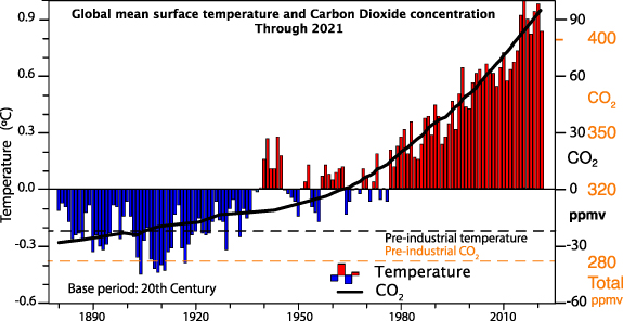
Figure 1. Estimated changes in annual global mean surface temperatures (°C, color bars) and CO2 concentrations (thick black line) over the past 150 years relative to twentieth century average values. Carbon dioxide concentrations since 1957 are from direct measurements at Mauna Loa, Hawaii, while earlier estimates are derived from ice core records. The scale for CO2 concentrations is in parts per million by volume (ppm), relative to the twentieth century mean of 333.7 ppm, while the temperature anomalies are relative to a mean of 14 °C. Also given as dashed values are the preindustrial estimated values, where the value is 280 ppm, with the scale in orange at right for carbon dioxide. Reproduced from Trenberth and Fasullo (2013). © 2013 The Authors. CC BY-NC-ND 3.0.
Download figure:
Standard image High-resolution imageThe EEI is arguably the most important metric related to climate change. It is the net result of all the processes and feedbacks in play in the climate system. However, it is also important to recognize the components of radiation at TOA, the absorbed solar radiation (ASR) and net outgoing longwave radiation (OLR). The ASR is the net incoming after reflected radiation is accounted for and varies with clouds. The net EEI is the ASR-OLR. A key reason for this breakdown relates to proposed geoengineering, in particular, so-called solar radiation management (SRM), a euphemistic name if ever there was one (Trenberth 2022). SRM alters ASR while the problem is trapping of OLR. In between are all the weather systems and hydrological cycle.
The radiative heat is variously transferred into sensible heat (related to temperatures), latent energy (related to changes in phase of water), potential energy (related to gravity and height), and kinetic energy (related to movement), and the richness of the phenomena and transformations among these various forms of energy are what makes this problem both challenging and interesting scientifically.
It is not (yet) possible to measure EEI directly, although changes measured from satellites are believed to be reliable, albeit biased. The only practical way to estimate net EEI is through an inventory of the changes in energy.
2. Assessing EEI
In our assessment of the EEI, the focus is on the well observed period from 2005 to 2019 (see section 3). The EEI is about 460 TW or globally 0.90 ± 0.15 W m−2 (Trenberth 2022). This can be compared with the net ASR and OLR of about 240 W m−2 as an estimate of the flow-through energy. Consequently, the EEI is very small and cannot be directly discerned or measured. Nevertheless, it is very large compared with estimated direct human influences such as the total electricity generated globally (about 5.7 TW in 2018) (Trenberth 2022).
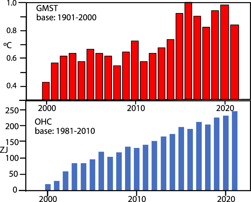
About 93% of the extra heat from the EEI ends up in the ocean as increasing ocean heat content (OHC). In 2022, the global OHC was the highest on record (Cheng et al 2022) and the global warming signal in OHC is large compared with the natural variability, unlike GMST, so that trends in OHC can be detected in four years (Cheng et al 2018), see figure 2 for example. The second-best signal-to-noise ratio is in the related sea level rise (SLR), as about 40% comes from OHC and the associated expansion of the ocean, while the rest mainly comes from melting of land ice: glaciers, Greenland, Antarctica that puts more water into the ocean. For SLR the trend detection occurs in about five years while for GMST the trend detection requires more than two decades (Cheng et al 2018).

Figure 2. For 2000–2021, GMST as in figure 1, and corresponding OHC in zettajoules relative to a baseline mean for 1981–2010, based on Cheng et al (2022).
Download figure:
Standard image High-resolution imageOn average nearly 3% of the EEI goes into melting ice and another 4% goes into raising temperatures of land and melting permafrost, while less than 1% remains in the atmosphere. The changes in GMST relate to those on land and sea surface temperatures (SSTs) in the ocean, and the increase in GMST (figure 1) is a consequence. The primary reasons for these distributions of excess heat relate to the heat capacity of these climate system components, the specific heat of water versus land versus air, and the masses involved; see Trenberth (2022) for a comprehensive review.
However, the initial excess energy has profound effects and big impacts along the way to its destination. The radiative energy is mostly absorbed at the surface where it mainly contributes to increased evaporation and moistening of the atmosphere, and is eventually realized as latent heating of the atmosphere during precipitation. This invigorates the hydrological cycle. In regions where it is not raining, it leads to enhanced drying then heating, increasing risk of heat waves and wildfires on land. It increases intensity of droughts. The evaporated moisture, carried by the atmosphere, converges into storms and associated frontal systems, where it increases precipitation rates, increasing risk of flooding on land. The latent heat released may also intensify some weather systems such as hurricanes and convection (thunderstorms). The warmer moister air is more buoyant and, helped by many weather phenomena, it rises and expands in lower pressures and cools adiabatically, then spreads out maybe thousands of km away and warms as it subsides, thus redistributing energy often to higher and drier regions where it can radiate to space.
In general, all components of the climate system react to heating by trying to get rid of excess heat in one way or another. The most effective method overall globally is radiative cooling as higher temperatures increase radiation by the fourth power of absolute temperature. Moreover, unequal heating leads to gradients that drive instabilities in the atmosphere (convective, baroclinic) and mixing is pervasive. In the ocean, warmer waters and those with lower salinity are less dense, and thermohaline circulations may develop, although most ocean currents are driven by winds. In ice and land, energy may be redistributed by water flows or conduction, but the latter is a very inefficient process.
In the ocean, heating occurs from the top down; warm on top of colder water is a stable configuration so that the stability and stratification of the ocean increase (Li et al 2020). Whereas globally, GMST and SSTs have clearly increased since about the 1970s (figure 1), for deeper ocean layers there is a delay that increases with depth. Globally, the top 500 m of the ocean are clearly warming since 1980, for 500–1000 m depth since 1990, 1000–1500 m layer since 1998, and from 1500 to 2000 m since 2005 (Cheng et al 2021). Indeed, it is a major challenge for climate models to get this heat penetration right, since it depends on unresolved sub-grid scale processes like mixing and convection, and how well or whether tidal mixing is included. A preliminary check of CMIP6 models reveals too much heating of the deep ocean (too large diffusion) but too little heating of the layers given above. This ocean heat redistribution is a factor in climate sensitivity of models and the errors contribute to too much surface warming.
The GMST was the fifth or sixth warmest on record in 2021 (depends on the dataset), in part, because of the year-long La Niña conditions, in which cool conditions in the tropical Pacific influence weather patterns around the world. Under those conditions the ocean stores extra heat, and then releases heat during El Niño events, making El Niño years like 1998 and 2016 relatively the warmest on record while OHC declines a small but measurable amount. There is also a signal in SLR because more rain occurs over the ocean in El Niño and droughts are more common over land, while more rains and snows occur on land in La Niña events. In the La Niña event in 2011 the extensive rains and snows, especially over North America, Siberia, and Australia (where it led to revival of Lake Eyre) took 5 mm of water out of the global ocean (Boening et al 2012).
There is a lot more natural variability in surface air temperatures than in ocean temperatures because of El Niño/La Niña and weather events (figure 2). For the oceans, the natural variability on top of warming creates hot spots locally, sometimes called 'marine heat waves,' that vary from year to year but are increasing (Tanaka et al 2022). Those hot spots have profound influences on marine life, from tiny plankton to fish, marine mammals, and seabirds. Other hot spots eventually result in more activity in the atmosphere, such as hurricanes (Trenberth et al 2018) which then take heat out of the ocean even as some is also mixed deeper.
All five oceans are warming (Cheng et al 2022), with the largest amounts of warming in the Atlantic Ocean and Southern Ocean surrounding Antarctica. That is a concern for Antarctica's ice as warmer waters can creep under Antarctica's ice shelves, thinning them and resulting in calving off huge icebergs.
3. EEI observations
So how well is EEI known and does it matter? The discussion above makes the point that it matters a lot. Knowing how much extra energy affects weather systems and rainfall is vital to understand the increasing weather extremes. Moreover, because those weather events move energy around and help the climate system get rid of energy by radiating it to space, these processes also affect the rise in GMST. In other words, they affect the nature and magnitude of climate change, and have major implications for how well the outcomes can be modeled and predicted.
Climate prediction is based upon comprehensive Earth system models that include modules for the atmosphere, oceans, land, and cryosphere. In the atmosphere such models are used for numerical weather prediction (NWP), and these are now quite sophisticated and enable reliable predictions about ten days in advance, following comprehensive analysis of continual atmospheric observations (over 200 million per day; NOAA 2022) using four-dimensional-data assimilation. Beyond that time frame, chaotic elements destroy deterministic forecasts, but the climate may be projected through knowledge of the interactions with the land, oceans, and ice, which are the main energy reservoirs.
There are good estimates of TOA radiation variations from Clouds and Earth's Radiant Energy System (CERES) (Loeb et al 2018) since March 2000 (figure 3). The exact calibration is not well known because of questions about sampling, especially clouds, but it is thought that the changes throughout the time series are reasonably reliable. In figure 3 the zero is set based upon OHC estimates (Loeb et al 2018). There is an apparent trend in the CERES EEI (Loeb et al 2021) of 0.4 W m−2 decade−1 for March 2000–December 2021. This trend is mainly due to an increase in ASR associated with decreased reflection by reduced Arctic sea-ice, and changes in clouds, reduced aerosols and increases in GHGs.
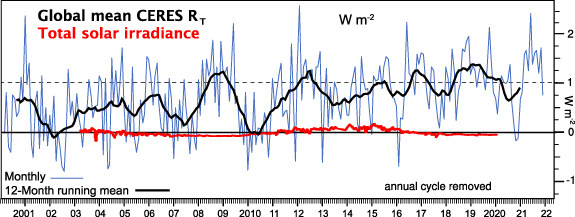
Figure 3. Monthly time series of CERES EBAF Ed4.1 net radiation at the TOA (positive down) relative to an estimated mean of 0.7 W m−2 for 2000–2015 (see Loeb et al (2018)) (blue). The mean annual cycle is removed, and the heavy black line is the 12 month running mean (includes data through 2021). The total solar irradiance contribution is in red (updated, see Coddington et al (2016)) with the mean (1361 W m−2) removed, and converted to a radiative forcing by dividing by 4 and multiplying by 0.7 to account for the albedo.
Download figure:
Standard image High-resolution imageThe Sun is often invoked as a possible source of climate change but contributions from changes in the Sun (figure 3) are very small. All energy from the oceans, land and ice must go through the atmosphere to reach the TOA, and the standard deviation of annual mean TOA net radiation is about three times that of the atmospheric energy tendency (figure 4), highlighting that it is not atmospheric energy or temperatures so much as clouds that cause the TOA variability (Trenberth (2022) for details).

Figure 4. Times series of 12 month running means of CERES TOA radiation (black) along with total atmospheric energy change (orange), land estimate (brown) and ocean heat content changes from two sources (green and light blue). The inset gives average values for all components including land (brown) and ice (blue) in W m−2 for 2005–2019. The thin black line is zero. Updated from Trenberth (2022).
Download figure:
Standard image High-resolution image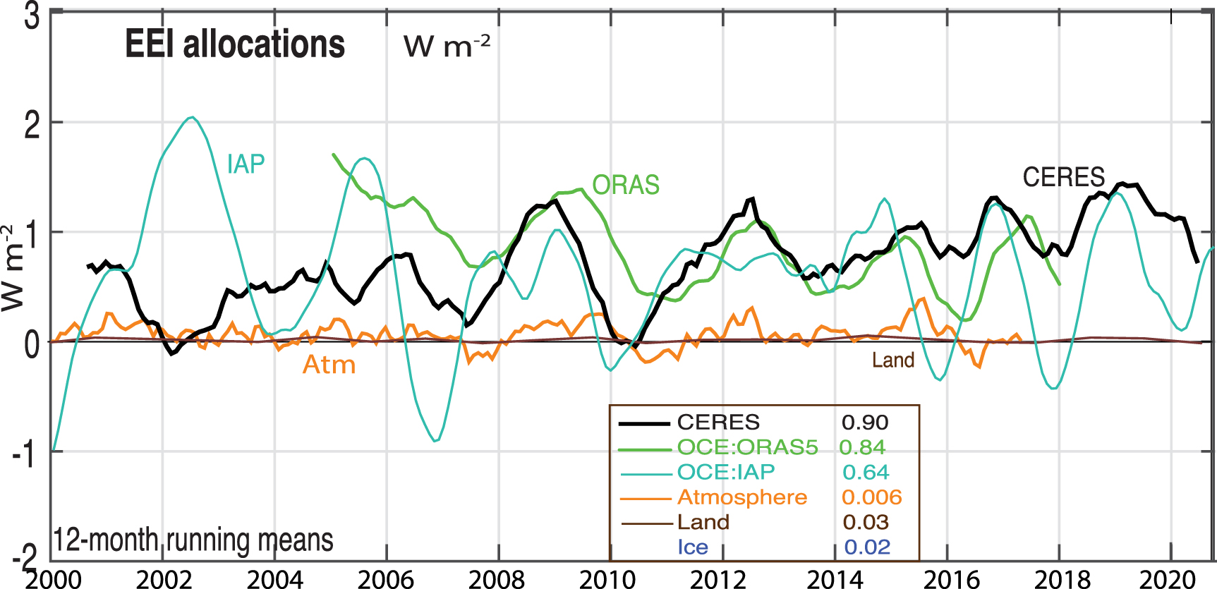
Many estimates of EEI exist. Trenberth et al (2009) made an estimate based upon atmospheric energy and surface fluxes. Trenberth (2009) estimated contributions from other components of the climate system, something that was done more thoroughly by Hansen et al (2011), and von Schuckmann et al (2016) provided a good review of the outstanding issues.
Changes in atmospheric energy are well known (figure 4) from atmospheric reanalyses. For the land, there are no such time series except right at the surface, where the extreme heterogeneity of the land surface in terms of topography, rocks, soil, vegetation and water distributions provides major challenges. Rough estimates of overall land heating below the surface come from boreholes, made for other purposes. Here a time series for land based on land surface air temperatures for a layer of 10 m is estimated. Highest value is in 2015 of 0.05 W m−2 (figure 4).
The situation is only slightly better for ice. Time series exist for sea ice area, and an estimate exists of Arctic sea ice volume (updated from Schweiger et al (2011)), while appraisals continue to be made of how much ice remains in glaciers. Maximum values for Arctic sea ice melt occur in 2008, 2011 and 2016 of 0.03 W m−2. Estimates of changes in Greenland and Antarctica by different means exist but their uncertainties are large enough that error bars may not overlap (Trenberth 2022).
Modeling of the oceans has progressed, and the ocean observing system made major advances in the early 2000s with the deployment of the Argo array of over 3000 profiling floats that sample the upper 2000 m of the ocean for temperature and salinity. Estimates exist of OHC changes since 1958, the International Geophysical Year, although uncertainties are large prior to 2005. Two ocean OHC datasets have been used in figure 4. ORAS5 is constrained by altimetry observations of sea level and surface fluxes, but values are too high prior to 2008 when Argo reached full depth coverage and are less reliable after 2015 when it went operational. The IAP dataset has spurious variability related to sampling as it lacks the surface flux constraint. A preliminary newer ORAS construction (not shown) more closely matches IAP from 2006 to 2010.
In figure 4, the estimated inventory of the mean values for 2005–2019 are given. The ice time series is too small to be seen and the land values barely emerge in 2015 and 2019. Ideally, it should be possible to add up the contributions from all sources and they should agree with CERES. In figure 4 the agreement is reasonable from 2010 to 2016.
The ability to close the TOA energy budget beyond a long-term average is improving but remains a limitation on how well it is possible to analyze what is going on in the climate system and why. However, using physical constraints, regional energy balances and transports at 1000 km scales can be achieved (Trenberth and Zhang 2019). Desirably, all data should be assimilated into a comprehensive Earth system model and each component initialized, to provide the starting point for predictions, as done in NWP. Such experimental predictions for seasons in advance exist. The failure and indeed inability of models to match observations in the ocean, land and ice domains demonstrates their limitations, but short-term predictions are potentially a way forward to challenge and improve both models and observations.
It is vital to understand the net energy gain, and how much and where heat is redistributed within the Earth system. How much heat might be moved to where it can be purged from the Earth via radiation to limit warming? Utilizing the EEI framework, the relevant observations and their synthesis challenges models and highlights needed improvements, but with prospects for major payoffs from better information about what is going on, and why, and what the outlook is for the future.
Acknowledgments
Many thanks to John Fasullo for processing the CERES EBAF data Ed4.1, available from https://ceres.larc.nasa.gov/data/. NCAR is sponsored by the U.S. National Science Foundation.
Data availability statement
All data that support the findings of this study are included within the article (and any supplementary information files).